Tutorial 2: Ranking LOMs and Predicting Loaded Shifts

Tutorial 1 fit each lumped oscillator model (LOM) to a single, strongly and asymmetrically coupled device. Here, we’ll see how to construct LOMs for a variety of parameters and test their accuracy under loading.

In this tutorial we will see how to:

1. Rank the accuracy of LOMs. We rank all three LOMs (Foster, Analytical, and Optimized) against the CPW circuit model over a grid of coupling capacitances.

2. Predict a frequency shift from capacitive loads. We attach capacitive loads to a fitted device and check that its (L, C) reproduce the shifted CPW frequency — not just the bare resonance.

This helps you see whether the LOM that you have chosen is capable of standing in for a resonator inside a larger network with arbitrary loads.

Setup

For the setup we will first construct the same \(7000\) um CPW as in Tutorial 1:

import warnings
warnings.filterwarnings("ignore")

import numpy as np
import pandas as pd
import matplotlib.pyplot as plt
import skrf as rf
from scipy.signal import find_peaks

import simpleLOMs as sl

sl.apply_style()   # one shared simpleLOMs figure style


cpw    = sl.CPWParams(ep_r=11.45)                    # substrate
coarse = rf.Frequency(4e9, 12e9, 8_001, unit="Hz")   # fit grid
Ctog   = 1e-14
Z0     = 50.0
d      = 7.0e-3                                      # 7 mm lambda/2, f0 ~ 7.5-8 GHz
MODELS = ("optimized", "foster", "analytical")       # best first

We will test the performance of all three available lumped element models in this tutorial.

MODELS = ("optimized", "foster", "analytical")       # best first

In order to use the Analytical expression, we need \(f_{bare}\) and the line impedance, which we’ll compute as part of the setup.

f_bare = sl.bare_cpw_resonance_hz(d, cpw_params=cpw)   # unloaded lambda/2 resonance
z_line = sl.cpw_line_impedance(cpw, f_hz=f_bare)       # line impedance
print(cpw)
print(f"bare-line f_r = {f_bare/1e9:.4f} GHz,  line impedance = {z_line:.2f} ohm")

CPWParams(w=1.17e-05, s=5.1e-06, t=0.0, h=0.0005, rho=1e-19, ep_r=11.45, has_metal_backside=False, tand=0.0)
bare-line f_r = 8.5830 GHz,  line impedance = 46.43 ohm

1. Ranking the LOMs across the coupling plane

Tutorial 1 ranked the models at a single strongly-coupled device (\(C_{c1}=30\), \(C_{c2}=70\) fF). Here we rank them across the whole plane: a grid of coupling capacitances \((C_{c1}, C_{c2})\) from 15 fF (weak) to 150 fF (very strong), allowing them to differ — real devices couple asymmetrically to input and output.

At each grid point, we measure the CPW ground-truth \((f_0, \kappa)\) with extract_f0_kappa, fit each LOM with fit_lom — handing the Optimized fit a window sized to the measured linewidth, since at 150 fF the resonance is the better part of a GHz wide and fit_lom’s default internal window cannot bracket it — then rebuild each model through its own ``get_network()``, circle-fit \(f_0\), and record the signed percent error \(\delta f_0 / f_0\). The Analytical model is anchored to the bare-line frequency and line impedance printed above — the same anchoring Tutorial 1 used — so its errors here are genuinely the closed form’s, not an artifact of feeding it an already-loaded frequency.

Note: this is a deliberately small grid (9 Optimized fits) so the notebook executes in about three minutes. Feel free to increase N to map the plane in more detail.

N = 3                                          # grid points per axis (N x N Optimized fits)
cc = np.geomspace(15e-15, 150e-15, N)
f0_err = {m: np.full((N, N), np.nan) for m in MODELS}   # [row=Cc2, col=Cc1]

for i, Cc2 in enumerate(cc):
    for j, Cc1 in enumerate(cc):
        f0c, kc = sl.extract_f0_kappa(cpw, d, Cc1=Cc1, Cc2=Cc2, Ctog=Ctog, Z0=Z0, n_fine=8001)
        # evaluation window sized to the (broad, at strong coupling) linewidth
        half = max(0.8e9, 5 * kc)
        fr = rf.Frequency(max(1e9, f0c - half), f0c + half, 8_001, unit="Hz")
        for m in MODELS:
            fit_freq = fr if m == "optimized" else coarse
            mod = sl.fit_lom(d, model=m, Cc1=Cc1, Cc2=Cc2, Ctog=Ctog, Z0=Z0,
                             cpw_params=cpw, freq=fit_freq, return_model=True)
            net = mod.get_network(fr, Cc1=Cc1, Cc2=Cc2, Ctog1=Ctog, Ctog2=Ctog, Z0=Z0)
            # Probe the stronger port — same convention as extract_f0_kappa
            # under asymmetric coupling.
            port = 0 if Cc1 >= Cc2 else 1
            f0m, km = sl.circle_fit_f0_kappa(net, port, port)
            f0_err[m][i, j] = 100.0 * (f0m - f0c) / f0c
        print(f"Cc1={Cc1*1e15:5.1f} Cc2={Cc2*1e15:5.1f} fF | "
              + "  ".join(f"{sl.MODEL_LABELS[m]}: {f0_err[m][i, j]:+.3f}%" for m in MODELS),
              flush=True)

# summary: |delta f0| statistics per model
summary = pd.DataFrame(
    {sl.MODEL_LABELS[m]: [np.abs(f0_err[m]).min(), np.median(np.abs(f0_err[m])), np.abs(f0_err[m]).max()]
     for m in MODELS},
    index=["min |df0| (%)", "median |df0| (%)", "max |df0| (%)"],
)
summary

Cc1= 15.0 Cc2= 15.0 fF | Optimized: -0.000%  Foster: +0.037%  Analytical: +0.069%
Cc1= 47.4 Cc2= 15.0 fF | Optimized: -0.001%  Foster: +0.110%  Analytical: +0.161%
Cc1=150.0 Cc2= 15.0 fF | Optimized: +0.060%  Foster: +0.335%  Analytical: +0.432%
Cc1= 15.0 Cc2= 47.4 fF | Optimized: -0.001%  Foster: +0.110%  Analytical: +0.161%
Cc1= 47.4 Cc2= 47.4 fF | Optimized: -0.004%  Foster: +0.232%  Analytical: +0.299%
Cc1=150.0 Cc2= 47.4 fF | Optimized: +0.045%  Foster: +0.579%  Analytical: +0.690%
Cc1= 15.0 Cc2=150.0 fF | Optimized: +0.060%  Foster: +0.335%  Analytical: +0.432%
Cc1= 47.4 Cc2=150.0 fF | Optimized: +0.045%  Foster: +0.579%  Analytical: +0.690%
Cc1=150.0 Cc2=150.0 fF | Optimized: -0.002%  Foster: +1.462%  Analytical: +1.614%

	Optimized	Foster	Analytical
min |df0| (%)	0.000042	0.036749	0.068749
median |df0| (%)	0.003654	0.335301	0.431841
max |df0| (%)	0.060479	1.461949	1.613534

We can now plot the error maps (on a log color scale, since the models differ by orders of magnitude). The star marks Tutorial 1’s device.

fig, axes = sl.plot_heatmaps(
    cc * 1e15, cc * 1e15,
    {sl.MODEL_LABELS[m]: np.abs(f0_err[m]) for m in MODELS},
    xlabel=sl.axis_label("Coupling", r"C_{c1}", "fF"),
    ylabel=sl.axis_label("Coupling", r"C_{c2}", "fF"),
    cbar_label=r"$|\delta f_0/f_0|$  (%)",
    norm="log",
    show=False,
)
for k, ax in enumerate(np.atleast_1d(axes)):
    ax.plot(30, 70, marker="*", ms=13, mfc="w", mec="0.15", mew=0.9, ls="none")
    if k == 0:
        ax.annotate("Tut. 1", (30, 70), xytext=(4, 5), textcoords="offset points",
                    color="w", fontsize=9)
plt.show()

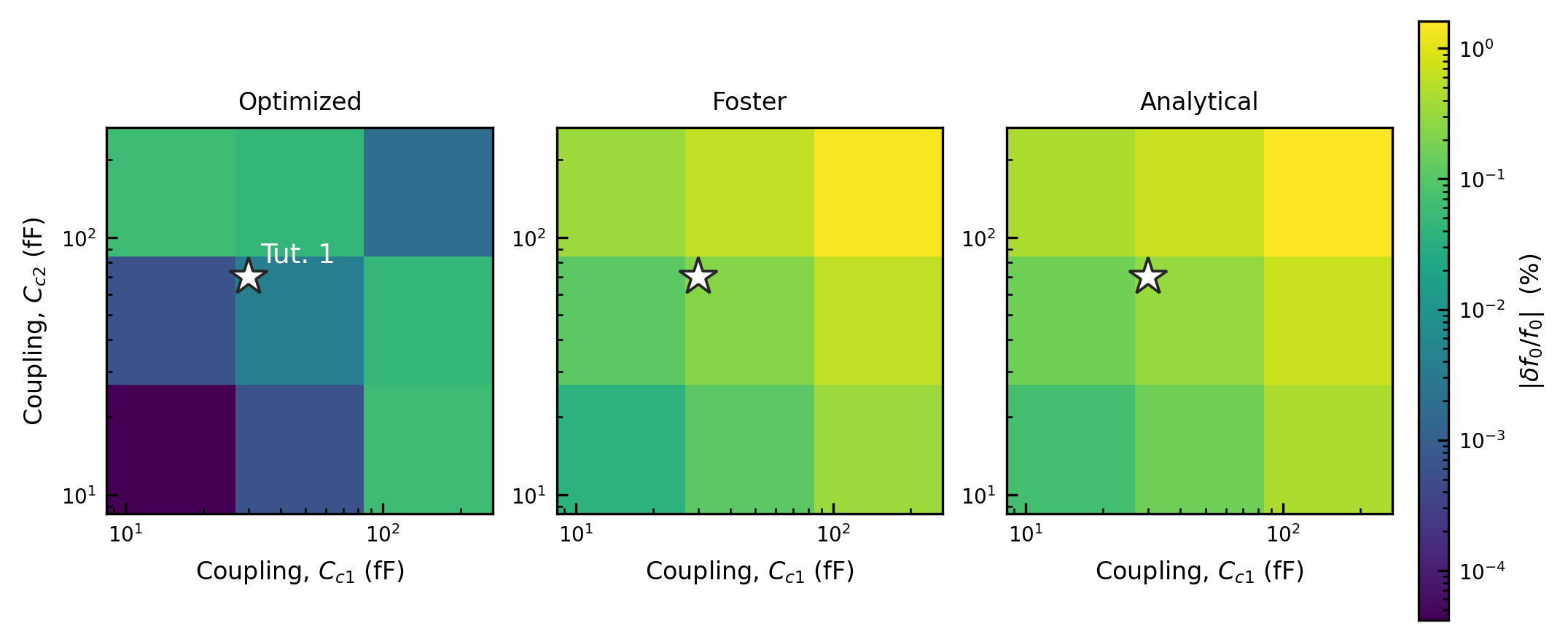
The Optimized method tracks the CPW to a few thousandths of a percent over most of the plane — never worse than \(0.06\%\), at the strongly asymmetric corners (15 fF against 150 fF) — while the other two, which do not inherently incorporate the loading, do not.

The Foster and Analytical errors instead grow with the total coupling, reaching \(\approx 1.5\%\) at the strongest symmetric point (150 fF on both ports).

2. Predicting the loaded frequency shift

The point of a fitted (L, C) is to stand in for the resonator when something else is attached to it. So to test this we attach a load and ask whether each model reproduces how far the CPW resonance moves.

For this part of the tutorial we’ll choose just one device, strong, asymmetric regime (\(C_{c1}=60\), \(C_{c2}=35\) fF) and add a 100 fF shunt capacitor on each side — the kind of capacitive loading a neighbouring element presents. The loaded topology (drawn below) probes the circuit through weak cc_port capacitors (1 fF by default, exposed as a parameter of the loaded builders), so the measured resonance belongs to the resonator + coupling + load, not to the 50 \(\Omega\) terminations.

Measure bare and loaded the same way. The bare reference is the same weak-probe topology with a negligible load, so the shift

\[\Delta f = f_0^{\text{loaded}} - f_0^{\text{bare}}, \qquad \epsilon = \frac{\Delta f_{\text{LC}} - \Delta f_{\text{CPW}}}{\Delta f_{\text{CPW}}}\]

isolates the load’s effect. (If you instead compared against the 50 \(\Omega\)- terminated bare device of Part 1, the change of probe convention alone would move \(f_0\) by more than the load does — always difference two measurements of the same circuit convention.) With a clean convention the physics reads off directly: a shunt-capacitor load adds capacitance, so it pulls the resonance down.

Cc1, Cc2 = 60e-15, 35e-15          # strong, asymmetric design point
Cload = 100e-15                    # shunt-capacitor load on each port side
L_OPEN = 1.0e3                     # open the load inductor -> capacitor-only load
C_NEG = 1e-21                      # negligible load capacitance -> "bare" reference

from pathlib import Path
figdir = Path("figures")
figdir.mkdir(exist_ok=True)
sch = sl.cpw_loaded_schematic_2port(
    d, Cc1, Cc2, Ctog, Ctog, L_OPEN, Cload, L_OPEN, Cload,
    cpw_params=cpw, freq=coarse, Z0=Z0,
    annotations={"load": "100 fF shunt (inductor opened)", "probe": "cc_port = 1 fF"},
    title="Loaded CPW resonator, weak-probe convention",
)
sch.save_svg(figdir / "tut02_loaded_topology.svg")
sch.save_html(figdir / "tut02_loaded_topology.html")
print("saved figures/tut02_loaded_topology.svg|.html")
sch

saved figures/tut02_loaded_topology.svg|.html

We first fit all three models on the bare, 50-ohm terminated device.

def measure_f0(build):
    """Locate a resonance by its |S21| peak (wide grid), then circle-fit f0 on a
    fine local grid. Robust for the sharp, weakly-probed resonances here."""
    wide = rf.Frequency(5.0e9, 9.5e9, 9_001, unit="Hz")
    f_approx = wide.f[np.argmax(np.abs(build(wide).s[:, 1, 0]))]
    fine = rf.Frequency(f_approx - 60e6, f_approx + 60e6, 20_001, unit="Hz")
    f0, _ = sl.circle_fit_f0_kappa(build(fine), 0, 0)
    return f0

models = {m: sl.fit_lom(d, model=m, Cc1=Cc1, Cc2=Cc2, Ctog=Ctog, Z0=Z0,
                        cpw_params=cpw, freq=coarse, return_model=True)
          for m in MODELS}

Now we can determine the shift in frequency when comparing the bare and loaded CPWs. This acts as the ground truth for the comparsion.

b_cpw = lambda fr, C1, C2: sl.cpw_resonator_loaded_network_2port(
    fr, d, Cc1, Cc2, Ctog, Ctog, L_OPEN, C1, L_OPEN, C2, cpw_params=cpw, Z0=Z0)
f0_cpw_bare = measure_f0(lambda fr: b_cpw(fr, C_NEG, C_NEG))
f0_cpw_load = measure_f0(lambda fr: b_cpw(fr, Cload, Cload))
df_cpw = f0_cpw_load - f0_cpw_bare

def lc_builder(m, mod):
    if m == "optimized":
        return lambda fr, C1, C2: sl.lc_resonator_loaded_network_2port(
            mod.L, mod.C, Cc1, Cc2, L_OPEN, C1, L_OPEN, C2, freq=fr, Z0=Z0)
    return lambda fr, C1, C2: sl.lc_resonator_loaded_network_with_grounds_2port(
        mod.L, mod.C, Cc1, Cc2, Ctog, Ctog, L_OPEN, C1, L_OPEN, C2, freq=fr, Z0=Z0)

rows = [{"model": "CPW (truth)", "f0_bare_GHz": f0_cpw_bare / 1e9,
         "f0_loaded_GHz": f0_cpw_load / 1e9, "shift_MHz": df_cpw / 1e6,
         "loaded_err_MHz": 0.0, "shift_err_%": 0.0}]
for m in MODELS:
    b = lc_builder(m, models[m])
    fb = measure_f0(lambda fr: b(fr, C_NEG, C_NEG))
    fl = measure_f0(lambda fr: b(fr, Cload, Cload))
    df = fl - fb
    rows.append({"model": sl.MODEL_LABELS[m], "f0_bare_GHz": fb / 1e9,
                 "f0_loaded_GHz": fl / 1e9, "shift_MHz": df / 1e6,
                 "loaded_err_MHz": (fl - f0_cpw_load) / 1e6,
                 "shift_err_%": 100.0 * (df - df_cpw) / df_cpw})

loaded = pd.DataFrame(rows).set_index("model")
print(f"100 fF loads pull the CPW resonance {df_cpw/1e6:+.1f} MHz "
      f"({f0_cpw_bare/1e9:.4f} -> {f0_cpw_load/1e9:.4f} GHz)")
loaded.round(4)

100 fF loads pull the CPW resonance -387.1 MHz (8.4354 -> 8.0484 GHz)

	f0_bare_GHz	f0_loaded_GHz	shift_MHz	loaded_err_MHz	shift_err_%
model
CPW (truth)	8.4354	8.0484	-387.0558	0.0000	0.0000
Optimized	8.4469	8.0487	-398.2113	0.3463	2.8822
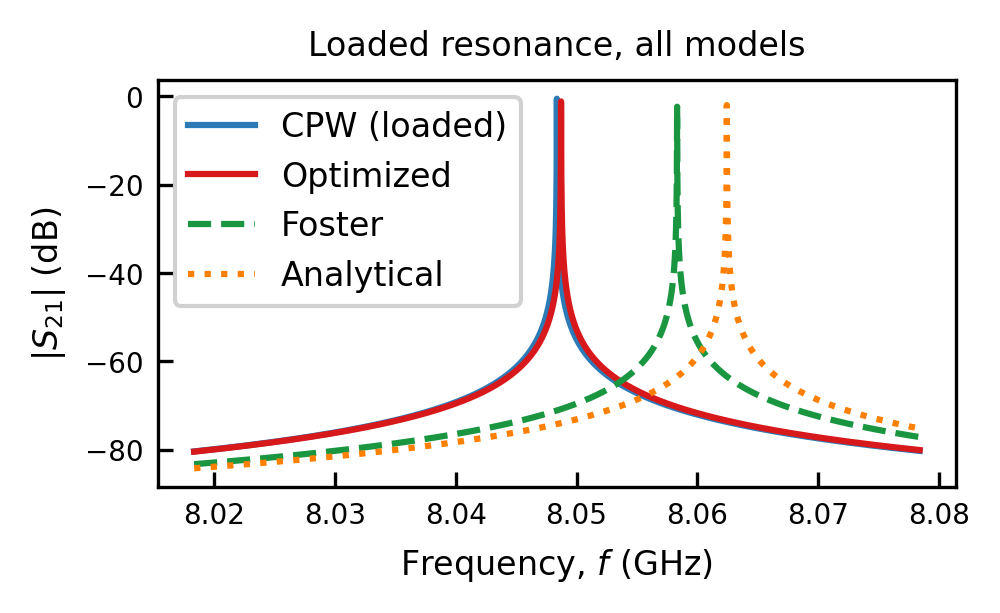
Foster	8.4354	8.0583	-377.0917	9.9430	-2.5743
Analytical	8.4366	8.0624	-374.2112	14.0569	-3.3185

Now we can compare the bare vs loaded CPW resonance.

wide = rf.Frequency(7.7e9, 8.8e9, 12_001, unit="Hz")
s_db = lambda net: 20 * np.log10(np.abs(net.s[:, 1, 0]))
sl.plot_curves(
    None,
    (wide.f / 1e9, s_db(b_cpw(wide, C_NEG, C_NEG)), "CPW bare", dict(color="0.6", lw=1.6)),
    (wide.f / 1e9, s_db(b_cpw(wide, Cload, Cload)), "CPW loaded", dict(color="0.1", lw=1.6)),
    xlabel=sl.LABEL_FREQ,
    ylabel=r"$|S_{21}|$ (dB)",
    vline=[f0_cpw_bare / 1e9, f0_cpw_load / 1e9],
)
print(rf"Delta f = {df_cpw/1e6:+.1f} MHz")

# Zoom on the loaded resonance: each LOM vs the CPW ground truth.
W = rf.Frequency(f0_cpw_load - 30e6, f0_cpw_load + 30e6, 12_001, unit="Hz")
nets = {"CPW (loaded)": b_cpw(W, Cload, Cload)}
for m in MODELS:
    nets[sl.MODEL_LABELS[m]] = lc_builder(m, models[m])(W, Cload, Cload)
sl.plot_all_models(nets, m=1, n=0, quantity="db", title="Loaded resonance, all models")

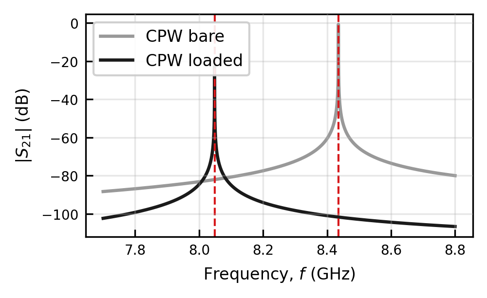
Delta f = -387.1 MHz

(<Figure size 1012.5x625.759 with 1 Axes>,
 <Axes: title={'center': 'Loaded resonance, all models'}, xlabel='Frequency, $f$ (GHz)', ylabel='$|S_{21}|$ (dB)'>)

As we expect, the Optimized model is the best at predicting how the element will behave in a distributed network.