Tutorial 6: From a Lumped Oscillator Model to readout parameters
Tutorials 1 and 2 fit a lumped L–C model to a CPW resonator and check how accurately it reproduces the full distributed response.
In this tutorial, you will learn how to turning that L and C into quantities you might actually use for designing a superconducting circuit. We will use the two helpers, resonator_readout_params and extract_f0_kappa, to do the following:
Convert a fitted model into a resonance frequency \(f_r\), characteristic impedance \(Z_r\), and zero-point voltage and current fluctuations
Measure the loaded linewidth \(\kappa\) and get the quality factor \(Q\)
Design a symmetric \(C_c\) to match a target \(Q\)
[ ]:
import warnings
warnings.filterwarnings("ignore")

import numpy as np
import matplotlib.pyplot as plt
import skrf as rf

import simpleLOMs as sl

sl.apply_style()
1. Fit a resonator and read off its L and C
We use a 7 mm CPW resonator on an ultracold-silicon chip. The fit_lom(d, model=...) returns effective L and C for any of the three models ("optimized", "foster", "analytical"). In this tutorial, we use Optimized, which is the default and the most accurate. However, you can switch MODEL below if you want a faster Foster or Analytical fit.
[3]:
cpw = sl.CPWParams(ep_r=11.45)                       # ultracold-silicon substrate
freq = rf.Frequency(4e9, 12e9, 8001, unit="Hz")

MODEL = "optimized"                               # or "foster" / "analytical"
L, C = sl.fit_lom(7e-3, model=MODEL, cpw_params=cpw, freq=freq)

print("Fitted lumped model ({}):".format(MODEL))
print("  L = {:.4f} nH".format(L * 1e9))
print("  C = {:.2f} fF".format(C * 1e15))
Fitted lumped model (optimized):
  L = 0.5605 nH
  C = 633.14 fF
2. Convert fitted L, C to relevant circuit parameters.
One of the benefits of lumped oscillator models is that they can be easily used to convert to Hamiltonian parameters using standard circuit quantization techniques.
2a. Unloaded quantities
To convert L, C to frequency, impedance, and zero-point fluctuations, use resonator_readout_params(L, C) to get these values based on the fitted L, C quantities.
\(Z_r\) and the zero-point fluctuations depend only on L and C, so we can compute them before saying anything about loss or coupling.
[4]:
rp = sl.resonator_readout_params(L, C)
print(rp.summary())
Resonator readout parameters
----------------------------
  f_r        =     8.4486 GHz
  Z_r        =      29.75 Ohm
  L          =     0.5605 nH
  C          =   633.1379 fF
  V_zpf      =      2.103 uV
  I_zpf      =     70.667 nA
\(V_\mathrm{zpf}\) is on the order of a few \(\mu\)V and \(I_\mathrm{zpf}\) is on the order of tens of nA, as expected for a standard coplanar readout resonator.
2b. Loaded quantities (\(\kappa\), \(Q\))
The quality factor \(Q\) is not a property of the bare mode. Instead it is set by how strongly we couple the mode to the environment.
In this geometry, the coupling capacitor \(C_c\) ties the resonator to the 50 \(\Omega\) feedline and gives the mode a finite linewidth. We measure it using a circle fit via extract_f0_kappa, which locates the resonance on a coarse grid, then re-simulates a narrow window on a fine grid and reads \(f_0\) and \(\kappa\) from a circle fit (a single wide grid cannot resolve a sub-MHz linewidth).
Beginning with a 6 fF coupling capacitor, we’ll extract \(f_0\) and \(\kappa\) fo the CPW system.
[ ]:
Cc = 6e-15
f0, kappa = sl.extract_f0_kappa(cpw, d=7e-3, Cc=Cc)
print("measured:  f0 = {:.4f} GHz    kappa/2pi = {:.4f} MHz".format(f0/1e9, kappa/1e6))
measured:  f0 = 8.3697 GHz    kappa/2pi = 2.4586 MHz

Resonator readout parameters
----------------------------
  f_r        =     8.4486 GHz
  Z_r        =      29.75 Ohm
  L          =     0.5605 nH
  C          =   633.1379 fF
  V_zpf      =      2.103 uV
  I_zpf      =     70.667 nA
  kappa/2pi  =     2.4586 MHz
  Q (loaded) =       3436
  tau_photon =       64.7 ns
2c. Summarize the results
[ ]:
rp = sl.resonator_readout_params(L, C, kappa_Hz=kappa)
print()
print(rp.summary())
Because this chip is lossless (tand = 0, superconducting metal), the internal quality factor is effectively infinite and the loaded \(Q\) is set entirely by the coupling — i.e. here \(Q \approx Q_c\), the coupling quality factor. On a real device the loaded \(Q\) combines with the internal \(Q_i\) as \(Q_\ell^{-1} = Q_c^{-1} + Q_i^{-1}\).
The photon lifetime \(\tau = 1/(2\pi\kappa) \approx 65\) ns is the readout resonator’s ring-down time.
[ ]:
3. Setting a design to match a target parameter.
Here we will use the example of showing how the coupling capacitor \(C_c\) sets \(\kappa\) and \(Q\) to show how you can use sweeps like this to correlate geometric features of your circuit design to actual desired parameters.
3a. Set up the sweep
We’ll use 8 Cc values with all else fixed, and use extract_f0_kappa to get \(\kappa\) an subsequently \(Q\)
[6]:
Cc_values = np.linspace(2e-15, 16e-15, 8)
f0s, kappas, Qs = [], [], []
for Cc in Cc_values:
    f0, kappa = sl.extract_f0_kappa(cpw, d=7e-3, Cc=Cc)
    rp = sl.resonator_readout_params(L, C, kappa_Hz=kappa)
    f0s.append(f0 / 1e9)
    kappas.append(kappa / 1e6)
    Qs.append(rp.Q)

f0s, kappas, Qs = map(np.array, (f0s, kappas, Qs))
for cc, k, q in zip(Cc_values, kappas, Qs):
    print("Cc = {:4.1f} fF    kappa/2pi = {:7.3f} MHz    Q = {:8.0f}".format(cc*1e15, k, q))
Cc =  2.0 fF    kappa/2pi =   0.279 MHz    Q =    30272
Cc =  4.0 fF    kappa/2pi =   1.104 MHz    Q =     7656
Cc =  6.0 fF    kappa/2pi =   2.459 MHz    Q =     3436
Cc =  8.0 fF    kappa/2pi =   4.328 MHz    Q =     1952
Cc = 10.0 fF    kappa/2pi =   6.696 MHz    Q =     1262
Cc = 12.0 fF    kappa/2pi =   9.547 MHz    Q =      885
Cc = 14.0 fF    kappa/2pi =  12.865 MHz    Q =      657
Cc = 16.0 fF    kappa/2pi =  16.636 MHz    Q =      508
3b. (Optional) Validate the data
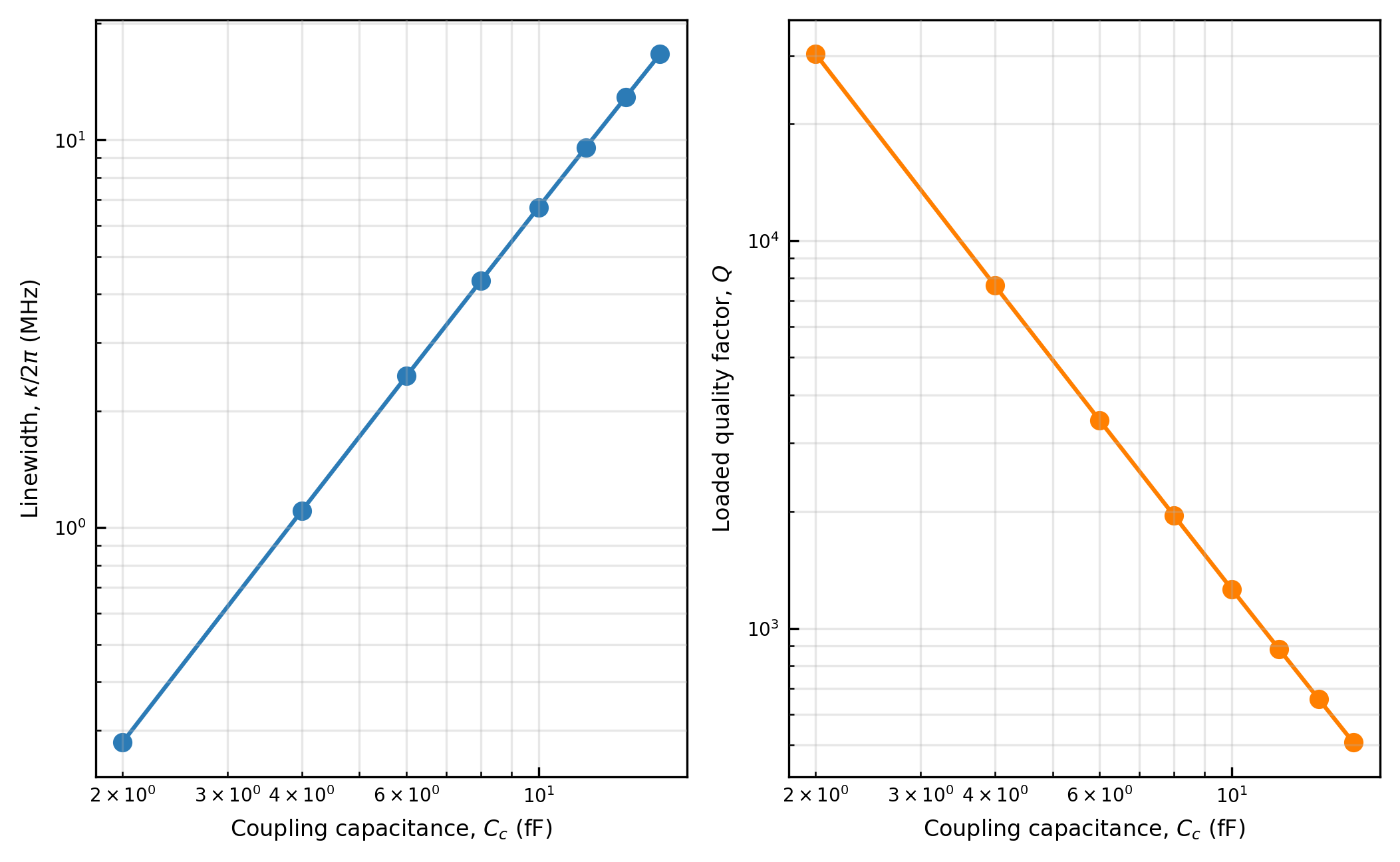
We already know approximately what to expect from this data based on approximate formulas. For a capacitively coupled resonator we expect that expectation is \(\kappa \propto C_c^2\) and therefore \(Q \propto 1/C_c^2\). To ensure that this pattern occured, we can plot the two of them in log scale:
[7]:
sl.plot_curve_pair(
    Cc_values * 1e15, kappas, Qs,
    xlabel=sl.LABEL_CC,
    ylabel0=sl.LABEL_KAPPA,
    ylabel1=sl.axis_label("Loaded quality factor", "Q"),
    xscale="log", yscale="log",
)
[7]:
(<Figure size 2117.1x1308.44 with 2 Axes>,
 array([<Axes: xlabel='Coupling capacitance, $C_c$ (fF)', ylabel='Linewidth, $\\kappa/2\\pi$ (MHz)'>,
        <Axes: xlabel='Coupling capacitance, $C_c$ (fF)', ylabel='Loaded quality factor, $Q$'>],
       dtype=object))
Indeed the graph matches our expectations. To quantify it, we can fit a line in log-log space.
[ ]:
slope_k = np.polyfit(np.log(Cc_values), np.log(kappas), 1)[0]
slope_Q = np.polyfit(np.log(Cc_values), np.log(Qs), 1)[0]
print("kappa  ~  Cc^{:+.2f}   (expected +2)".format(slope_k))
print("Q      ~  Cc^{:+.2f}   (expected -2)".format(slope_Q))
kappa  ~  Cc^+1.97   (expected +2)
Q      ~  Cc^-1.97   (expected -2)
The fitted exponents sit close to \(\pm 2\), confirming that \(\kappa\) and \(Q\) scale with \(C_c\) as expected.
This fitted curve is now the curve we can design against. WE can pick the \(C_c\) that lands the readout resonator at the \(\kappa\) (equivalently \(Q\)) we want.
3c. Reading off a coupling for a target \(Q\)
Because \(Q\) is monotonic in \(C_c\), you can interpolate the sweep to size the coupling capacitor for a chosen quality factor. Here, let’s set the target \(Q\) to be \(5000\).
[ ]:
target_Q = 5000
Cc_target = sl.invert_monotonic(Cc_values, Qs, target_Q, log=True)
print("For a loaded Q of {}, choose  Cc ~ {:.2f} fF".format(target_Q, Cc_target * 1e15))
For a loaded Q of 5000, choose Cc ~ 4.96 fF
Now as described in Tutorial 4, we can invert the \(Cc\) graph to match the target.
[ ]:
Cc_target = sl.invert_monotonic(Cc_values, Qs, target_Q, log=True)
print("For a loaded Q of {}, choose  Cc ~ {:.2f} fF".format(target_Q, Cc_target * 1e15))
We now have a way to convert lumped parameters into design targets.
Next up
In Tutorial 7 we will learn how to use these principles taught in this tutorial to hit a target frequency and target \(Q\) simultaneously by choosing the resonator length and coupling together.