Tutorial 4: Parameter sweeps of CPW and LOM designs

While the primary purpose of the simpleLOMs pacakge is to construct lumped models of superconducting devices, another aspect of this package is its ability to test a wide variety of device geometries at the circuit level, including the length, coupling, or the CPW cross-section.

In this tutorial, we will see how to perform parameter sweeps of both CPW and lumped designs using extract_f0_kappa , fit_lom, and resonator_readout_params. By the end you will be able to sweep any device parameter of the network and extract a circuit that fits a desired design parameter.

import warnings
warnings.filterwarnings("ignore")

import dataclasses
import numpy as np
import matplotlib.pyplot as plt
import skrf as rf

import simpleLOMs as sl


# Shared simpleLOMs figure style — one identical look across every tutorial.
sl.apply_style()

cpw = sl.CPWParams(ep_r=11.45)                        # ultracold-silicon substrate
freq = rf.Frequency(4e9, 12e9, 8001, unit="Hz")
MODEL = "optimized"                                # best / default LOM

Parameter sweeps with measure_sweep

sl.measure_sweep(values, measure) is a function to perform a parameter sweep for an arbitrary knob in the design of a device, including geometry fields that are not SweepConfig attributes.

Sweep 1: Resonator length sweep for frequency

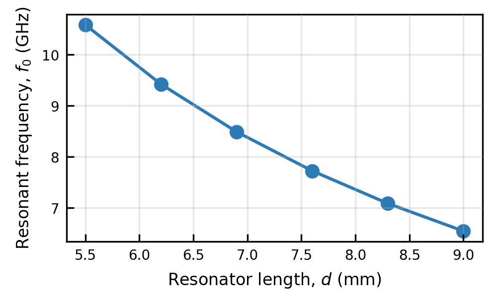
The resonator length has a disproportionately large impact on the frequency of the CPW and as such it acts as the coarse frequency knob.

d_values = np.linspace(5.5e-3, 9.0e-3, 6)          # 5.5 - 9.0 mm
r1 = sl.measure_sweep(d_values, lambda d: {"f0_GHz": sl.extract_f0_kappa(cpw, d=d, Cc=6e-15)[0] / 1e9})

for d, f in zip(r1["value"], r1["f0_GHz"]):
    print("d = {:.2f} mm    f0 = {:.4f} GHz".format(d * 1e3, f))

d = 5.50 mm    f0 = 10.5807 GHz
d = 6.20 mm    f0 = 9.4195 GHz
d = 6.90 mm    f0 = 8.4879 GHz
d = 7.60 mm    f0 = 7.7240 GHz
d = 8.30 mm    f0 = 7.0863 GHz
d = 9.00 mm    f0 = 6.5459 GHz

sl.plot_curves(
    r1["value"] * 1e3, r1["f0_GHz"],
    xlabel=sl.LABEL_LENGTH,
    ylabel=sl.LABEL_F0,
    fmt="o-",
    color=sl.COLOR_PRIMARY,
)

(<Figure size 1012.5x625.759 with 1 Axes>,
 <Axes: xlabel='Resonator length, $d$ (mm)', ylabel='Resonant frequency, $f_0$ (GHz)'>)

Sweep 2: Coupling sweep for linewidth and \(Q\)

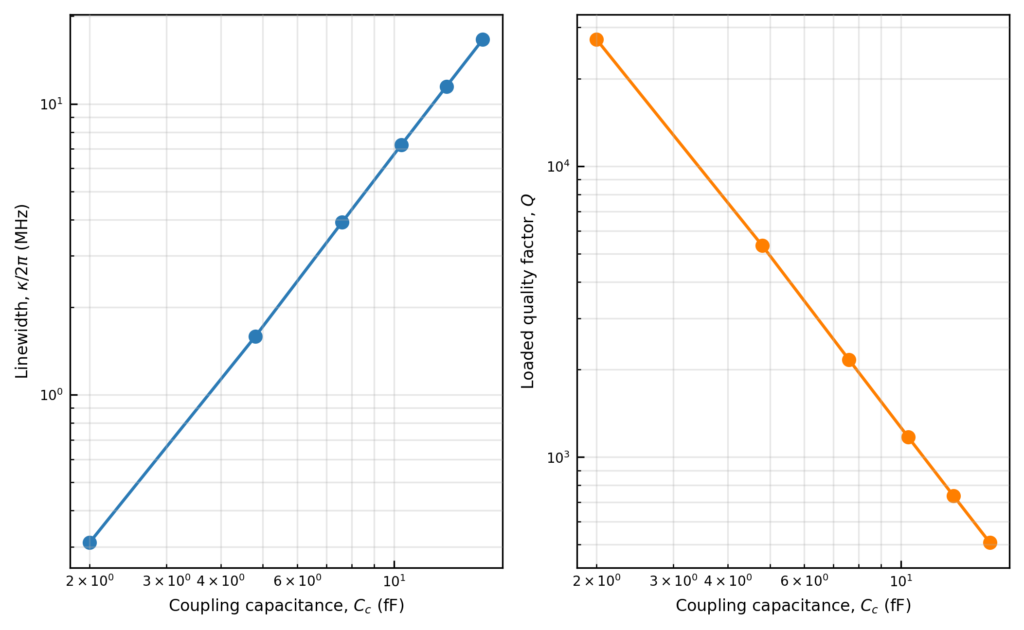
Once an approximate desired frequency has been reached, length may be kept fixed, and the user can now tune the coupling capacitor \(C_c\) to change the linewidth.

d0 = 7e-3
L, C = sl.fit_lom(d0, model=MODEL, cpw_params=cpw, freq=freq)   # one fit, reused below

def measure_coupling(Cc):
    f0, kappa = sl.extract_f0_kappa(cpw, d=d0, Cc=Cc)
    rp = sl.resonator_readout_params(L, C, kappa_Hz=kappa)
    return {"kappa_MHz": kappa / 1e6, "Q": rp.Q}

Cc_values = np.linspace(2e-15, 16e-15, 6)
r2 = sl.measure_sweep(Cc_values, measure_coupling)

for Cc, k, q in zip(r2["value"], r2["kappa_MHz"], r2["Q"]):
    print("Cc = {:4.1f} fF    kappa/2pi = {:7.3f} MHz    Q = {:8.0f}".format(Cc * 1e15, k, q))

Cc =  2.0 fF    kappa/2pi =   0.310 MHz    Q =    27259
Cc =  4.8 fF    kappa/2pi =   1.583 MHz    Q =     5339
Cc =  7.6 fF    kappa/2pi =   3.914 MHz    Q =     2160
Cc = 10.4 fF    kappa/2pi =   7.228 MHz    Q =     1169
Cc = 13.2 fF    kappa/2pi =  11.483 MHz    Q =      736
Cc = 16.0 fF    kappa/2pi =  16.636 MHz    Q =      508

sl.plot_curve_pair(
    r2["value"] * 1e15, r2["kappa_MHz"], r2["Q"],
    xlabel=sl.LABEL_CC,
    ylabel0=sl.LABEL_KAPPA,
    ylabel1=sl.axis_label("Loaded quality factor", "Q"),
    xscale="log", yscale="log",
)

(<Figure size 2117.1x1308.44 with 2 Axes>,
 array([<Axes: xlabel='Coupling capacitance, $C_c$ (fF)', ylabel='Linewidth, $\\kappa/2\\pi$ (MHz)'>,
        <Axes: xlabel='Coupling capacitance, $C_c$ (fF)', ylabel='Loaded quality factor, $Q$'>],
       dtype=object))

Sweep 3: CPW geometry sweep

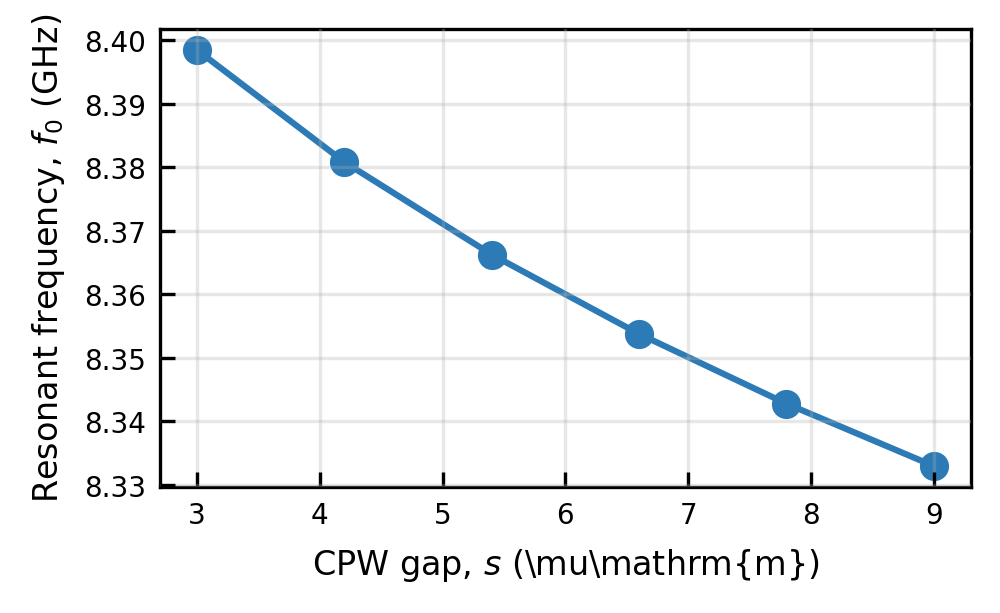
The value to be swept in measure_sweep can be either a circuit value (like in the previous examples) or a physical dimension. Here instead of sweeping a circuit value we instead sweep the CPW gap \(s\) by swapping it into CPWParams with dataclasses.replace, and measure the frequency the same way as Sweep 1.

s_values = np.linspace(3e-6, 9e-6, 6)              # gap 3 - 9 um
r3 = sl.measure_sweep(s_values, lambda sg: {
    "f0_GHz": sl.extract_f0_kappa(dataclasses.replace(cpw, s=sg), d=7e-3, Cc=6e-15)[0] / 1e9})

for sg, f in zip(r3["value"], r3["f0_GHz"]):
    print("s = {:.1f} um    f0 = {:.4f} GHz".format(sg * 1e6, f))

sl.plot_curves(
    r3["value"] * 1e6, r3["f0_GHz"],
    xlabel=sl.LABEL_CPW_GAP,
    ylabel=sl.LABEL_F0,
    fmt="o-",
    color=sl.COLOR_PRIMARY,
)

s = 3.0 um    f0 = 8.3985 GHz
s = 4.2 um    f0 = 8.3808 GHz
s = 5.4 um    f0 = 8.3663 GHz
s = 6.6 um    f0 = 8.3538 GHz
s = 7.8 um    f0 = 8.3428 GHz
s = 9.0 um    f0 = 8.3330 GHz

(<Figure size 1012.5x625.759 with 1 Axes>,
 <Axes: xlabel='CPW gap, $s$ (\\mu\\mathrm{m})', ylabel='Resonant frequency, $f_0$ (GHz)'>)

The gap moves \(f_0\) by only tens of MHz across this range, while the length moved it by more than a GHz in Sweep 1.

In a similar fashion, other parameters of geometry can be swept to reach target design parameters such as a desired frequency, without having to perform finite-element simulations. This concept is explored further in Tutorial 7.