Tutorial 9: Hybrid Series + Hanger Resonators
Tutorials 3 and 8 treat inline chains and hanger / notch resonators separately. But they may also be combined into one chain and analyzed as a whole.
In this tutorial, we will learn how to:
Construct a chain of resonators with both inline and hanger distributed CPWs.
Assemble a lumped system by fitting each piece with its respective LOM (
fit_lomfor the series resonator,fit_lom_hangerfor each hanger)Check the accuracy of the circuit model for the hybrid system.
For this tutorial, we will use the 3-resonator system:
[P1] -- Cc -- Ctog -- CPW_Purcell -- Ctog -- Cc --||-- hang1 -- hang2 -- [P2]
      \_____________ series / inline _____________/   \___ hangers ___/
It is also drawn later during the tutorial in hybrid_schematic_2port.
Setup
[ ]:
import warnings
warnings.filterwarnings("ignore")

import numpy as np
import pandas as pd
import matplotlib.pyplot as plt
import skrf as rf

import simpleLOMs as sl

sl.apply_style()
resonators: 1 inline Purcell (6.5 mm) + 2 open hangers [7.0, 8.0] mm
Our CPWs will all share a common CPWParams for the sake of this tutorial, but this can be changed in systems where the hybrid network has CPWs with different width or thickness.
[ ]:
cpw = sl.CPWParams(ep_r=11.45)
freq = rf.Frequency(5e9, 11e9, 4001, unit="Hz")
Z0 = 50.0
The series CPW, which we’ll refer to as the Purcell filter, uses the familiar inline topology.
[ ]:
d_purcell = 6.5e-3
Ccs_p = [8e-15, 8e-15]
Ctogs_p = [1e-14, 1e-14]
seg_purcell_cpw = [{"kind": "cpw", "d": d_purcell}]
THe inline resonator is then followed by two open hangers on a through feedline.
[ ]:
d_hangers = [7.0e-3, 8.0e-3]
Cc_taps = [30e-15, 30e-15]
seg_hangers_cpw = [
    {"kind": "cpw", "d": d, "termination": "open"} for d in d_hangers
]

print(f"resonators: 1 inline Purcell ({d_purcell*1e3:.1f} mm)"
      f" + {len(d_hangers)} open hangers {[d*1e3 for d in d_hangers]} mm")
1. Build the CPW hybrid (ground truth)
Build each block with its native network builder, then cascade them into one 2-port. The inline Purcell puts a transmission peak near its loaded resonance; each hanger puts a notch in \(|S_{21}|\).
1a. Network objects
[ ]:
purcell_cpw = sl.resonator_chain_network_2port(
    freq, seg_purcell_cpw, Ccs_p, Ctogs_p, cpw_params=cpw, Z0=Z0,
)
hangers_cpw = sl.hanger_resonator_network_2port(
    freq, seg_hangers_cpw, Cc_taps, cpw_params=cpw, Z0=Z0,
)
hybrid_cpw = purcell_cpw ** hangers_cpw
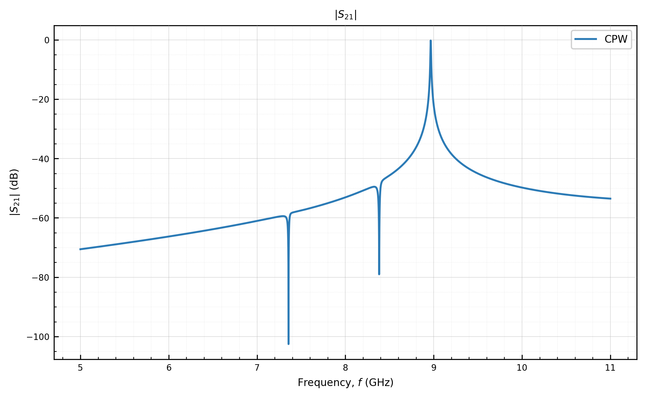
S21 peaks  (GHz): [7.2935 8.327  8.966 ]
S21 notches (GHz): [7.3565, 8.3825]
1b. Plot the network transmission
[ ]:
sl.plot_transmission({"CPW hybrid": hybrid_cpw}, m=1, n=0)

peaks_cpw = np.sort(sl.resonances_from_s_max(hybrid_cpw, m=1, n=0))
notches_cpw = sl.notches_below(hybrid_cpw, thresh=0.7)
print("S21 peaks  (GHz):", np.round(peaks_cpw / 1e9, 4))
print("S21 notches (GHz):", [round(f, 4) for f in notches_cpw])
As expected there are is one major peak and two notches visible on the graph.
2. Draw the hybrid schematic
hybrid_schematic_2port puts the inline Purcell and both hangers on one rail — the schematic counterpart of cascading the two networks. Same segment / capacitor arguments as the network builders.
[4]:
from pathlib import Path

figdir = Path("figures")
figdir.mkdir(exist_ok=True)

sch_cpw = sl.hybrid_schematic_2port(
    seg_purcell_cpw, Ccs_p, seg_hangers_cpw, Cc_taps,
    inline_Ctogs=Ctogs_p, cpw_params=cpw, freq=freq, Z0=Z0,
    annotations={"block": "hybrid CPW (Purcell + hangers)"},
)
sch_cpw.save_svg(figdir / "hybrid_cpw.svg")
sch_cpw.save_html(figdir / "hybrid_cpw.html")
print("saved figures/hybrid_cpw.svg|.html")
print("groups:", [g["label"] for g in sch_cpw.groups])
print("components:", [c.id for c in sch_cpw.components])
sch_cpw
saved figures/hybrid_cpw.svg|.html
groups: ['resonator 1', 'hanger 1', 'hanger 2']
components: ['P1', 'Cc1', 'Ctog1', 'TL1', 'Ctog2', 'Cc2', 'H1', 'H2', 'P2']
[4]:
3. Fit each resonator with the matching LOM
Inline Purcell:
fit_lom(..., model="optimized")against an isolatedCc -- Ctog -- CPW -- Ctog -- Ccsubgroup (Tutorial 3).Each hanger:
fit_lom_hangeragainst an isolated CPW hanger notch (Tutorial 8).
Fitting pieces in isolation (50 Ω ports / ideal feed) and stitching them back is the same approximation as Tutorial 3 — the hybrid test asks whether that still holds when the two topologies are cascaded.
3a. Inline fit
[ ]:
# --- Inline Purcell ---
sub_cpw = sl.cpw_resonator_network_2port(
    freq, d_purcell, Ccs_p[0], Ccs_p[1], Ctogs_p[0], Ctogs_p[1],
    cpw_params=cpw, Z0=Z0,
)
f0_sub, _ = sl.circle_fit_f0_kappa(sub_cpw, 0, 0)
fit_freq = rf.Frequency(f0_sub - 0.4e9, f0_sub + 0.4e9, 15_001, unit="Hz")

m_p = sl.fit_lom(
    d_purcell, model="optimized",
    Cc1=Ccs_p[0], Cc2=Ccs_p[1], Ctog1=Ctogs_p[0], Ctog2=Ctogs_p[1],
    cpw_params=cpw, freq=fit_freq, return_model=True,
)
print(f"Purcell (inline): d={d_purcell*1e3:.1f} mm  f0~{f0_sub/1e9:.3f} GHz  "
      f"L={m_p.L*1e9:.3f} nH  C={m_p.C*1e15:.2f} fF")
3b. Hanger fits
[ ]:
hanger_models = []
rows = [{
    "role": "Purcell (inline)",
    "topology": "series",
    "length_mm": d_purcell * 1e3,
    "L_nH": m_p.L * 1e9,
    "C_fF": m_p.C * 1e15,
}]
for i, (d, Cc) in enumerate(zip(d_hangers, Cc_taps), start=1):
    m = sl.fit_lom_hanger(
        d, Cc_tap=Cc, termination="open", cpw_params=cpw, return_model=True,
    )
    hanger_models.append(m)
    rows.append({
        "role": f"hanger {i}",
        "topology": "hanger",
        "length_mm": d * 1e3,
        "L_nH": m.L * 1e9,
        "C_fF": m.C * 1e15,
    })
    print(f"hanger {i}:          d={d*1e3:.1f} mm  "
          f"L={m.L*1e9:.3f} nH  C={m.C*1e15:.2f} fF")
Purcell (inline): d=6.5 mm  f0~8.966 GHz  L=0.523 nH  C=586.29 fF
hanger 1:          d=7.0 mm  L=0.553 nH  C=622.36 fF
hanger 2:          d=8.0 mm  L=0.632 nH  C=710.54 fF
| role | topology | length_mm | L_nH | C_fF | |
|---|---|---|---|---|---|
| 0 | Purcell (inline) | series | 6.5 | 0.523120 | 586.287145 |
| 1 | hanger 1 | hanger | 7.0 | 0.552535 | 622.361960 |
| 2 | hanger 2 | hanger | 8.0 | 0.632055 | 710.543203 |
3c. Inspect all fits
[ ]:
fits = pd.DataFrame(rows)
fits
4. Rebuild the lumped hybrid and compare to CPW
We now Cascade the inline \(L\), \(C\) and theHanger \(L\), \(C\)s generated in the previous step to build the overall netowrk which we will then overlay on \(|S_{21}|\).
[ ]:
seg_purcell_lc = [{"kind": "lc", "L": m_p.L, "C": m_p.C}]
seg_hangers_lc = [
    {"kind": "lc", "L": m.L, "C": m.C} for m in hanger_models
]

purcell_lc = sl.resonator_chain_network_2port(
    freq, seg_purcell_lc, Ccs_p, Ctogs=None, cpw_params=cpw, Z0=Z0,
)
hangers_lc = sl.hanger_resonator_network_2port(
    freq, seg_hangers_lc, Cc_taps, cpw_params=cpw, Z0=Z0,
)
hybrid_lc = purcell_lc ** hangers_lc
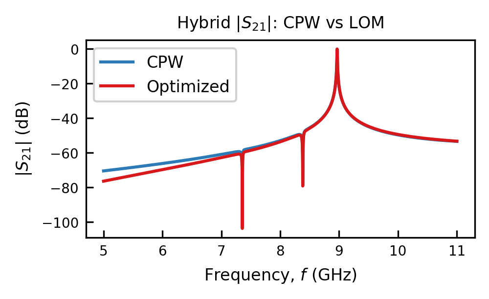
(<Figure size 1012.5x625.759 with 1 Axes>,
 <Axes: title={'center': 'Hybrid $|S_{21}|$: CPW vs LOM'}, xlabel='Frequency, $f$ (GHz)', ylabel='$|S_{21}|$ (dB)'>)
Plotting the transmission shows that there is strong agreement between the network of lumped elements and the fully distributed network:
[ ]:
sl.plot_all_models(
    {"CPW": hybrid_cpw, "Optimized": hybrid_lc},
    m=1, n=0, quantity="db",
    title=r"Hybrid $|S_{21}|$: CPW vs LOM",
)
4b. Evaluate the accuracy
With the two networks, to go further than just a graph we can determine numerically how accurate their predicted peaks are.
[7]:
notches_lc = sl.notches_below(hybrid_lc, thresh=0.7)
peaks_lc = np.sort(sl.resonances_from_s_max(hybrid_lc, m=1, n=0))

rows_n = []
for nc in notches_cpw:
    nl = min(notches_lc, key=lambda x: abs(x - nc))
    rows_n.append({
        "feature": "notch",
        "CPW_GHz": nc,
        "Lumped_GHz": nl,
        "error_MHz": (nl - nc) * 1e3,
        "error_%": 100.0 * (nl - nc) / nc,
    })

rows_p = []
for i, (pc, pl) in enumerate(zip(peaks_cpw[:3], peaks_lc[:3]), start=1):
    rows_p.append({
        "feature": f"peak {i}",
        "CPW_GHz": pc / 1e9,
        "Lumped_GHz": pl / 1e9,
        "error_MHz": (pl - pc) / 1e6,
        "error_%": 100.0 * (pl - pc) / pc,
    })

compare = pd.DataFrame(rows_n + rows_p)
print("Max |error_%|:", float(np.max(np.abs(compare["error_%"]))))
compare
Max |error_%|: 0.06169877287996161
[7]:
| feature | CPW_GHz | Lumped_GHz | error_MHz | error_% | |
|---|---|---|---|---|---|
| 0 | notch | 7.3565 | 7.3565 | 0.0 | 0.000000 |
| 1 | notch | 8.3825 | 8.3825 | 0.0 | 0.000000 |
| 2 | peak 1 | 7.2935 | 7.2980 | 4.5 | 0.061699 |
| 3 | peak 2 | 8.3270 | 8.3285 | 1.5 | 0.018014 |
| 4 | peak 3 | 8.9660 | 8.9660 | 0.0 | 0.000000 |
5. Lumped hybrid schematic
Same hybrid_schematic_2port, now with fitted LC tanks (no Ctog on the inline block — OptimizedFit absorbs grounds).
[8]:
sch_lc = sl.hybrid_schematic_2port(
    seg_purcell_lc, Ccs_p, seg_hangers_lc, Cc_taps,
    inline_Ctogs=None, cpw_params=cpw, freq=freq, Z0=Z0,
    annotations={"block": "hybrid LOM (OptimizedFit + HangerOptimizedFit)"},
)
sch_lc.save_svg(figdir / "hybrid_lc.svg")
sch_lc.save_html(figdir / "hybrid_lc.html")
print("saved figures/hybrid_lc.svg|.html")
sch_lc
saved figures/hybrid_lc.svg|.html
[8]: